The modules available for the attentional system were based on the selection model for perception proposed by Colombini (2016). This architecture incorporates several aspects of other related works and is capable of dealing with multiple sensory systems, multiple processes for feature extraction, decision-making and learning support.

1. Modules

1.1 - Bottom-up attention

During the bottom-up cycle, sensors provide external data stored in a time window in sensory memory to form feature maps.

1.2 - Top-down attention

In top-down interaction, the system receives changes from a cognitive block of individuality through the state of global attention and from another cognitive block of decision-making, interfering with the actuators, changing the environment, and thus again the entire system. This process depends on the objective of the system and the attentional dynamics of the current state: oriented, selective or sustained.

• Guided attention is the result of the attentional process to choose the focus of attention.
• Selective attention can emphasize specific features.
• Sustained attention is goal-driven. In biological systems, the endogenous component of attention begins 200 ms after the stimulus is attended to and remains as long as the task makes it necessary.

1.3 - Feature Maps

These maps are combined into a single combined feature map, which represents a weighted sum of the features.

1.4 - Salience Map

The combination of the feature map combined with the attentional map previously generated by the agent generates a saliency map, a representation of the environment perceived by the agent, modulated by the attentional process.

Through a selection of winners, for example, by a Winner-Takes-All algorithm, the most relevant stimulus in the saliency map can be defined.

1.5 - Inhibition of Return

The model also provides an inhibition system (IOR), which promotes the decay of the sensitivity of a region when there is a prolonged display of the stimulus, promoting attention to the next location with the second highest value in the saliency map. The succession of these events generates a sequential scan of the scene.

From the bottom-up perspective, only the most salient region of the resource combination will receive attention. As for the chronometry of the process, this feature or region will stimulate itself and its surroundings after a time t to another t + y. After this, the location or object feedback inhibition effect will compress the previously enhanced region for another period of time.

This modeling is based on the Gaussians illustrated bellow. The model considers the maximum and minimum contributions of attention lost over time, based on a usual curve adopted to model the integration of neuronal activity, and also describes the excitatory and inhibitory influence that will be demonstrated by attention in regions neighboring the Winner region. A process for the inhibition of a region maintained for a long time is also modeled, damaging the stimuli in the frequented location, allowing the orientation of attention to move away from goal maintenance.

Figure 1: Stimuli enhancement/decaying contribution over time. Typical curves for endogenous and exogenous lateral contribution; exogenous stimulus (with IOR); endogenous stimulus (without sustained attention); and successive endogenous stimulus (with sustained attention) and further impairment. Extracted from Colombini (2016)

2. Experiment

2.1 - Description

In the proposed example, the agent with the attentional system will see three objects with primary colors (red, green and blue).

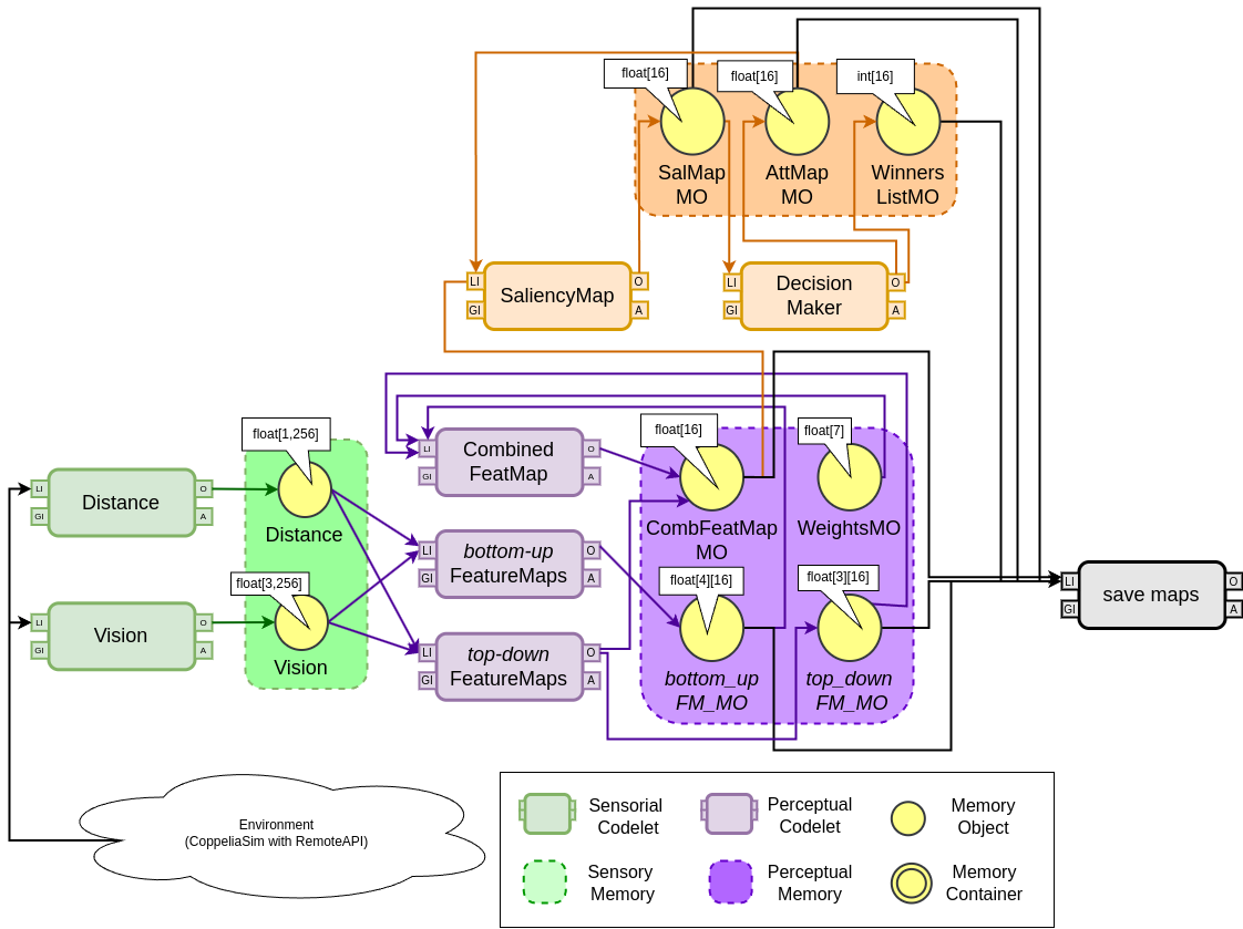
The classes that collect sensory data and the mechanisms that make up the attentional system were implemented with an agent with the CST cognitive tools in Java language with the following scheme.

Figure 2: Implementation scheme.

The main components are the AgentMind and OutsideCommunication classes. AgentMind is inherited from the Mind class, from CST, and adds Raw Memory and Coderack to form the cognitive system. AgentMind will be the creator of all memory objects (MOs) and codelets used. In turn, the OutsideCommunication class performs external communication with the robot through the RemoteAPI of the CoppeliaSim simulator.

For the SensorBufferCodelet, a generic method for deep copies was implemented, a term used for a copy created in a different location in memory, from the MOs related to sensory data. These copies are made through serializer objects in Java language. As the MemoryObject class, existing in the CST, already implements this interface, the information and functions stored in an instantiated MO also implement it.

Using feature maps codelets, the desired feature maps are constructed from sensory memory objects. Bottom-up and top-down maps compete for attention. Their memory objects are combined into a feature map combined by the codelet.

The functions that implement the IOR mechanism are based on temporal negative exponentials to generate a deterioration of attention over time. These mechanisms are regulated by constant parameters that influence the excitatory or inhibitory course of attention in bottom-up operation. The saliency map is obtained through the product between the combined feature map and the attentional map.

The attentional map is initialized with all its elements being equal to 1 and is fed back at each iteration by the Decision Making codelet. The saliency map influences the DecisionMaking codelet which is implemented according to a Winner-Takes-All approach, which defines the winning characteristic of each attentional cycle based on the inhibitory and excitatory cycles and promotes the change of the attentional map.

Figure 3: Adapted from Rossi (2021).

a) Image received through RemoteAPI. The axes represent the x and y coordinates of each pixel.

b) 256 regions used in calculating the feature maps for this work.

c) Illustration of the conversion 3D to 2D.

2.1.1 - Bottom-up Feature Maps

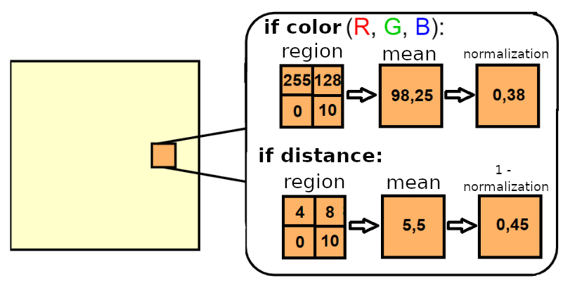
Figure 4: Example of extracting bottom-up feature maps. Each value of the feature maps (RGB) correspond to the averages and normalizations of the pixel values that belong to each region r_j. Each value in the distance feature map corresponds to 1 (one) minus the average normalized values of the pixels that belong to each region r_j. In the examples, for simplicity, each region is formed  by 2x2 pixels.  Adapted from Rossi (2021).

• F1. Red Channel. Represents the average of the vision sensor measurement values for the Red channel for each region. The bottom-up feature mapping function F1 is responsible for extracting information about the levels of red color in elements within the agent's field of vision attentive. Each element f1 of the F1 feature map, delimited to a region r, is acquired the mean array with the color levels for the channel Red. The mean array represents the calculated value for a given element f1 of the feature map F1.
• F2. Canal Green. Represents the average of the vision sensor measurement values for the Green channel for each region. The bottom-up feature mapping function F2 is responsible for extracting information about the levels of green color in the elements within the field of vision of the attending agent. Each element f2 of the F2 feature map, delimited to a region r, is acquired through the acquisition of the mean array with the color levels for the Green channel. The mean array represents the calculated value for a given element f2 of the feature map F2.
• F3. Channel Blue. Represents the average of the vision sensor measurement values for the Blue channel for each region. The bottom-up feature mapping function F3 is responsible for extract information about the levels of blue color in elements within the attentional agent's field of view. Each element f3 of the feature map F3, delimited to a region r, is obtained through the acquisition of the mean array in Algorithm 1 with the color levels for the Blue channel. The mean array represents the calculated value for a given element f3 of the F3 feature map.
• F4. Distance. Represents the average proximity based on the values of the relative distance measurements between obstacles and moving bodies and the attentional agent, with values in a range from 0 (closer) to 1 (farthest). The bottom-up feature mapping function F4 is responsible for extracting information about the arrangement of elements around the attentional agent. Each element f4 of the F4 feature map, delimited to a region r, is acquired through the acquisition of the mean array. The mean array represents the calculated value for a given element f4 of the F4 characteristics.

2.1.2 - top-down Feature Maps

The top-down feature mapping functions are responsible for extracting information about the arrangement of elements around the attentional agent;

Figure 5: Example of extracting Top-down feature maps of desired color and desired distance. Each character map value desired color characteristics is obtained by comparing the normalized averages of the pixel values which belong to each region r_j, in each of the RGB channels, with the desired color. The classification is carried out with the value furthest from the desired color. Each distance feature map value desired is obtained by comparing the normalized averages of the values of the pixels that belong to cents to each region r_j with the desired distance. In the examples, for simplicity, each region is formed  by 2x2 pixels.  Adapted from Rossi (2021).

 

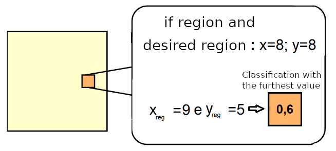
Figure 6: Extraction example of the top-down feature maps of the desired region. Each value of the desired region is obtained by comparing the average values of the coordinates of the pixels that belong to each region r_j with the coordinates of the desired region. Adapted from Rossi (2021).

• F5. Color-Objective. This characteristic represents the regions in which a desired color (with levels defined in three RGB channels) is highlighted and to which the agent's attention can be directed, in relation to the measurements of the vision sensor in each region.
• F6. Distance-Objective. This feature represents regions where a desired distance is highlighted and to which the agent's attention can be directed, in relation to distance measurements relative to the sensor in each region.
• F7. Region-Objective. This feature represents the regions of space to which attention of the agent can be directed, regardless of what is happening in that region.

2.1.3 - Combined Feature Map

The composite signal of all generated feature maps (bottom-up and top-down) is obtained according to the Colombini (2014) model, through the sum of the products between an element of the feature weight vector in the attentional system and a given feature map.

In order to classify the type of winning characteristic of the cycle (bottom-up or top-down) before applying the feedback inhibition algorithm, two values are obtained during the formation of the Combined Feature Map:

(i) the sum of the values generated by the bottom-up feature maps and

(ii) the sum of the values generated by the maps of top-down features.

If (i) > (ii), the winner of the attentional cycle is classified as bottom-up.

If (i) < (ii), the winner of the attentional cycle is classified as top-down

2.2 - Running the experiments

2.2.1 - Requirements

The code uses Java 11.

You must have Apache Netbeans and CoppeliaSim.

2.2.2 - Setup

1. Clone the repository https://github.com/leolellisr/attention_trail.
2. Open project CST_AttMod_App with Netbeans. Resolve any problems.
3. Clean and build the project.
4. Open CoppeliaSim and the scene training_obj.ttt present in folder scenes. Run it.

Figure 7: Scene used for the experiment.

5. Run the project on Netbeans.

2.2.3 - Stopping

You can stop the project after ~15 seconds. Stop first in Netbeans and then in CoppeliaSim.

2.2.4 - 1st run - Results

1. Images are stored in grayscale on folder /data. Sensor data, feature maps and attention maps are stored on folder /profile. Results are stored on folder /results. Create these folders if necessary.
2. Choose one image of folder data, copy its name without the format (after .). This will be our originally step.
3. Open the script map_att.py with a text editor.
4. Paste the name of the image on lines 297 to 318.
5. Run the script from folder /scripts
6. Usually the script run without problems. But if you have it, you will have to open the file that had the problem on folder /profile and copy the step closer to the originally step.
7. Results are stored on folder /results.

We have:

• Sensor maps

(a)	(b)	(c)	(d)

Figure 8: Sensor data.  (a) Vision sensor - channel red; (b) Vision sensor - channel green; (c) Vision sensor - channel blue; (d) depth.   

• feature maps

  • bottom-up

  (a)	(b)	(c)	(d)

  Figure 9: Bottom-up feature maps.  (a) Channel red; (b) Channel green; (c) Channel blue; (d) Depth.   

• top-down

(a)	(b)	(c)

Figure 10: Top-down feature maps.  (a) Desired distance (8 meters); (b) Desired color (blue); (c) Desired region (center).   

 

 

• Combined feature map

Figure 11: Combined feature map.

• Attention maps

(a)	(b)

Figure 12: Attention maps. (a) Attentional map; (b) Salience map.

 

2.2.4 - 2nd run - changing top-down fms

We can establish other values for the desired characteristics on the top-down feature maps.

1. Open the codelet of the top-down feature map that you want to change it. For example, TD_FM_Color.java, present on src/main/java/codelets/sensors.

2. Change the desired color from blue (0, 0, 255) to red (255, 0, 0). The channel intensities have to be establish with red_goal, green_goal and blue_goal variables.

3. Clean and build the project. Run the scene and the project again.

4. We will have changes on the maps: 

a. top-down color feature map

Figure 13: Top-down feature map - Desired color (Red).

b. Combined feature map

Figure 14: Combined feature map.

 

c. Salience map and Attention Map

(a)	(b)

Figure 15: Attention maps. (a) Salience Map; (b) Attentional map.